PyTorch Learning Series: Part 2
Continuing the PyTorch Learning Series! In this second part, we dive into Tensors in PyTorch and we get into some hands on coding to get to know tensors better!
 Sakalya Mitra
PyTorch Learning Series: Part 2
Hey Everyone! 👋 Welcome to the Part: 2 of the pytorch learning series.
I sincerely hope you all liked the Part 1 and gained the initial understanding of PyTorch.
Moving forward in the series, this part will be an in-depth discussion on Tensors in PyTorch
Here's the agenda of this blog:
- What are Tensors?
- Types of Tensors (Scalar, Vectors, Matrices, N-D Tensors)
- Why Tensors?
- Where are Tensors used in Deep Learning?
- Tensors in PyTorch - code based walkthrough on some important functions of tensors in PyTorch
Now that the agenda and plan is established, let's get going and start demistifying tensors
What are Tensors?
Tensors are a specialized multi-dimensional array designed for mathematical and computation efficiency
They are a generalization of scalars, vectors, and matrices, which are 0-dimensional, 1-dimensional, and 2-dimensional tensors, respectively.
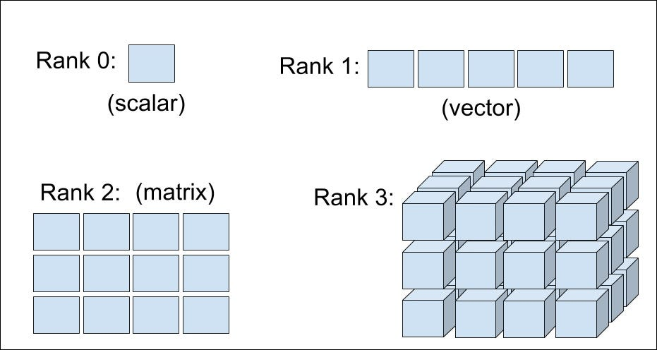
Apart from the these mostly used tensors, we can also represent other higher dimensional data using tensors.
Let's see some real world use cases where tensors are used
1. Scalars: 0-dimensional tensors
- They are typical a single number or value that are used for single metrics or constants
- An example would be the Loss value we get after a forward pass in a neural network. The loss function computes a single value which is ideally the difference between the actual and predicted label
2. Vectors: 1-dimensional tensors
- They represent a list or sequence of values
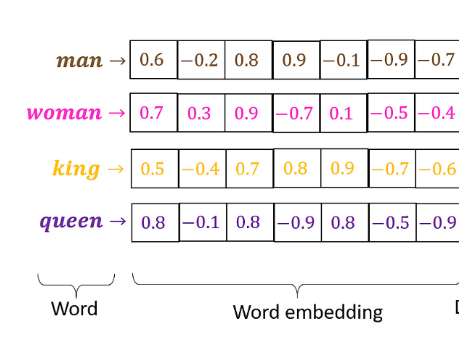
- An example would be feature vectors/ word embeddings in natural language processing. Each word in the sentence is represented as a 1D vector using embeddings
3. Matrices: 2-dimensional tensors
- This is essentially as 2D grid/sequence of numbers or values
- This is used to represent tabular or grid like data
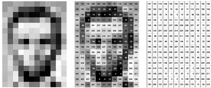
- An example for 2D tensors would be grayscale Images. A grayscale image can be represented as a 2D tensor where each entry corresponds to the pixel intensity
4. 3D Tensors
- These type of tensors add a third dimension over the 2D tensors to represent another dimension of information
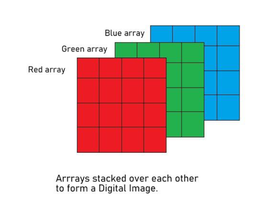
- For the previous Grayscale image example, adding another layer to the image pixel matrix would essentially mean representing coloured images
- A single coloured or RGB image is represented using a 3D tensor (width + height + channels)
- Example: The typical shape of RGB images used in Deep Learning tasks are [256, 256, 3] where the last dimension represent the colour channels.
5. 4D Tensors
- These are another higher dimensional tensors
- Continuing our Image example, it adds another layer of information which is the batch size
- Basically in deep learning tasks, most Conv Net models expect images as batches of data
- This means they process multiple RGB images in one epoch and those multiple images contruct one batch
- To represent the size of a batch, we use the 4th dimension
- Example: A batch of 32 images, each of size 128 x 128 having 3 channels can be represented as [32, 128, 128, 3] which is a 4D tensor
6. 5D Tensors
- These tensors are mainly used to add a time dimension over the 4D tensor
- It represents the data that changes over time ( video frames)
- For example, video data are the perfect examples of 5D tensors
- If we consider a video, it basically consists of a sequence of frames, where each frame is a RGB Image
- So if we consider a batch of 10 video clips, where each video clip has 16 frames each and each frame in turn has a 64 x 64 shape and have 3 channels. The tensor should would be [10, 16, 64, 64, 3].
These were some of the mostly used high dimensional tensors that we use in our day-to-day lives. We might also require some more higher-dimensional tensors in some fields but it is currently not in our scope of learning PyTorch and understanding tensors.
Now that we have an idea of what tensors are, the different types of tensors and their practical examples, its time to move on to our next section
Why are Tensors Useful?
Tensors provide various useful usecases that have made them a standalone choice in deep learning data representation.
- Mathematical Operations
- Tensors enable efficient mathematical computations (addition, multiplication, dot product, etc.) necessary for neural network operations.
- Representation of Real-world Data
- Data like images, audio, videos, and text can be represented as tensors:
- Images: Represented as 3D tensors (width x height x channels).
- Text: Tokenized and represented as 2D or 3D tensors (sequence length x embedding size).
- Video: Represented as 5D tensors
- Data like images, audio, videos, and text can be represented as tensors:
- Efficient Computations
- Tensors are optimized for hardware acceleration, allowing computations on GPUs or TPUs, which are crucial for training deep learning models.
- As tensors can run on GPUs, they are capable of parallel execution leading to very fast computations
- For example consider 2 matrices A = [[1,2],[3,4]] and B = [[5,6],[7,8]]. We are looking to perform elementwise addition in these 2 matrices.
- If it is being performed on a CPU, as it has a single core, each element-wise addition will take place in the same core sequentially one by one
- But the same process if run on the GPU, utilises the multiple-cores of GPU and performs the different element-wise additions on the individual cores parallely and provides faster computed results
Now it is quite clear to us the advantages of using Tensors and their applicability in Deep learning use cases. Let's now dive in to the last theoretical section of this blog before getting our hands on creating tensors and coding them out!
Where are Tensors used in Deep Learning?
We have discussed a lot about what tensors are, how they are useful. But where do we exactly use Tensors in Deep Learning is what we will explore here
- Data Storage
- Training data (images, text, etc.) is stored in tensors.
- As we already discussed in the first section, Image, Video, text data can be represented as Tensors
- Weights and Biases
- The learnable parameters of a neural network (weights, biases) are stored as tensors.
- When we train a neural network, there are a set of learnable parameters, weights & biases which are crucial for training the neural network. The weights and biases are normally represented as tensors as they are used for matrix operations and mathematical computations during forward and backward pass.
- Matrix Operations
- Neural networks involve operations like matrix multiplication, dot products, and broadcasting—all performed using tensors.
- The entities like weights, biases, inputs are all tensors and hence the matrix operations are computed using tensors only.
- Training Process
- During forward passes, tensors flow through the network.
- Gradients, represented as tensors, are calculated during the backward pass.
Tensor Hands-On
Well I am an ardent believer that until you get your hands dirty and actually implement stuff, there is no real learning. So let's jump right into it for Tensors!
Note: For this I used a free-tier Google Colab notebook and changed the runtime to T4 GPU available for free. Although it is based on availability , but even a normal CPU instance would be enough for this part as we will not be using any large data or complex operations that require a lot of memory or processing power.
First things first, let's import PyTorch and check the version we're working with:
import torch
print(torch.__version__)
Output
2.5.1+cu121
PyTorch can leverage the power of GPUs for faster computation. Let's check if we have a GPU available:
if torch.cuda.is_available():
    print("GPU is available!")
    print(f"Using GPU: {torch.cuda.get_device_name(0)}")
else:
    print("GPU not available. Using CPU.")
Output
GPU is available!
Using GPU: Tesla T4
Great! We have a Tesla T4 GPU available. This will significantly speed up our tensor operations when working with large datasets.
Creating a Tensor
Now let's explore the various ways to create tensors in PyTorch. Each method has its own use case depending on what you need.
Using torch.empty()
The empty() function creates an uninitialized tensor. This means the tensor will contain whatever garbage values were in that memory location - it's fast but unpredictable!
# using empty
a = torch.empty(2,3)
Let's verify the type of our newly created tensor:
# check type
type(a)
Output
torch.Tensor
Using torch.zeros() and torch.ones()
When you need tensors initialized with specific values, zeros() and ones() are your go-to functions. These are commonly used for initializing weights or creating masks.
# using zeros
torch.zeros(2,3)
Output
tensor([[0., 0., 0.],
        [0., 0., 0.]])
# using ones
torch.ones(2,3)
Output
tensor([[1., 1., 1.],
        [1., 1., 1.]])
Using torch.rand() for Random Values
Random tensors are essential for weight initialization in neural networks. The rand() function generates values from a uniform distribution between 0 and 1.
# using rand
torch.rand(2,3)
Output
tensor([[0.1192, 0.4828, 0.9105],
        [0.4266, 0.4203, 0.2719]])
Notice that if we run rand() again, we get completely different values:
# use of seed
torch.rand(2,3)
Output
tensor([[0.0064, 0.4451, 0.1580],
        [0.8119, 0.4629, 0.3227]])
Reproducibility with torch.manual_seed()
In machine learning, reproducibility is crucial. The manual_seed() function ensures you get the same random numbers every time you run your code:
# manual_seed
torch.manual_seed(100)
torch.rand(2,3)
Output
tensor([[0.1117, 0.8158, 0.2626],
        [0.4839, 0.6765, 0.7539]])
Let's verify - running the same seed again should give identical results:
torch.manual_seed(100)
torch.rand(2,3)
Output
tensor([[0.1117, 0.8158, 0.2626],
        [0.4839, 0.6765, 0.7539]])
Perfect! The values are exactly the same. This is incredibly useful when debugging or sharing your work with others.
Creating Tensors from Python Lists
You can also create tensors directly from Python lists or nested lists using torch.tensor():
# using tensor
torch.tensor([[1,2,3],[4,5,6]])
Output
tensor([[1, 2, 3],
        [4, 5, 6]])
Other Useful Tensor Creation Functions
PyTorch provides several specialized functions for common patterns:
# other ways

# arange - creates a sequence with a step value (like Python's range)
print("using arange ->", torch.arange(0,10,2))

# linspace - creates evenly spaced values between start and end
print("using linspace ->", torch.linspace(0,10,10))

# eye - creates an identity matrix (useful for linear algebra operations)
print("using eye ->", torch.eye(5))

# full - creates a tensor filled with a specific value
print("using full ->", torch.full((3, 3), 5))
Output
using arange -> tensor([0, 2, 4, 6, 8])
using linspace -> tensor([ 0.0000,  1.1111,  2.2222,  3.3333,  4.4444,  5.5556,  6.6667,  7.7778,
         8.8889, 10.0000])
using eye -> tensor([[1., 0., 0., 0., 0.],
        [0., 1., 0., 0., 0.],
        [0., 0., 1., 0., 0.],
        [0., 0., 0., 1., 0.],
        [0., 0., 0., 0., 1.]])
using full -> tensor([[5, 5, 5],
        [5, 5, 5],
        [5, 5, 5]])
Tensor Shapes
Understanding tensor shapes is fundamental when working with neural networks. Let's explore how to work with shapes and create tensors that match existing ones.
x = torch.tensor([[1,2,3],[4,5,6]])
x
Output
tensor([[1, 2, 3],
        [4, 5, 6]])
The .shape attribute tells us the dimensions of our tensor:
x.shape
Output
torch.Size([2, 3])
This tensor has 2 rows and 3 columns - a 2x3 matrix.
Creating Tensors with the Same Shape
Sometimes you need to create a new tensor that matches the shape of an existing one. PyTorch provides *_like() functions for this:
torch.empty_like(x)
Output
tensor([[     134842408414608,       96429401449888,     3503044046096754],
        [-2738188572259385344,  7020378893157883663,  8389754676633367105]])
⚠️ Notice those weird numbers? That's uninitialized memory! This is why
empty_like()should be used with caution.
For safer alternatives, use zeros_like() or ones_like():
torch.zeros_like(x)
Output
tensor([[0, 0, 0],
        [0, 0, 0]])
torch.ones_like(x)
Output
tensor([[1, 1, 1],
        [1, 1, 1]])
For random values, note that we need to specify the dtype since the original tensor was integers:
torch.rand_like(x, dtype=torch.float32)
Output
tensor([[0.4076, 0.6037, 0.9820],
        [0.0117, 0.3891, 0.5056]])
Tensor Data Types
PyTorch tensors have specific data types (dtypes) that affect precision, memory usage, and performance. Let's explore how to work with them.
Checking the Data Type
# find data type
x.dtype
Output
torch.int64
Specifying Data Type During Creation
You can explicitly set the data type when creating a tensor:
# assign data type
torch.tensor([1.0,2.0,3.0], dtype=torch.int32)
Output
tensor([1, 2, 3], dtype=torch.int32)
Notice how the float values were converted to integers!
torch.tensor([1,2,3], dtype=torch.float64)
Output
tensor([1., 2., 3.], dtype=torch.float64)
Converting Data Types with .to()
The .to() method is a flexible way to convert tensor types (and also move them between CPU and GPU):
# using to()
x.to(torch.float32)
Output
tensor([[1., 2., 3.],
        [4., 5., 6.]])
Common PyTorch Data Types Reference
Here's a comprehensive table of all available data types:
| Data Type | Dtype | Description |
|---|---|---|
| 32-bit Floating Point | torch.float32 | Standard floating-point type used for most deep learning tasks. Provides a balance between precision and memory usage. |
| 64-bit Floating Point | torch.float64 | Double-precision floating point. Useful for high-precision numerical tasks but uses more memory. |
| 16-bit Floating Point | torch.float16 | Half-precision floating point. Commonly used in mixed-precision training to reduce memory and computational overhead on modern GPUs. |
| BFloat16 | torch.bfloat16 | Brain floating-point format with reduced precision compared to float16. Used in mixed-precision training, especially on TPUs. |
| 8-bit Floating Point | torch.float8 | Ultra-low-precision floating point. Used for experimental applications and extreme memory-constrained environments (less common). |
| 8-bit Integer | torch.int8 | 8-bit signed integer. Used for quantized models to save memory and computation in inference. |
| 16-bit Integer | torch.int16 | 16-bit signed integer. Useful for special numerical tasks requiring intermediate precision. |
| 32-bit Integer | torch.int32 | Standard signed integer type. Commonly used for indexing and general-purpose numerical tasks. |
| 64-bit Integer | torch.int64 | Long integer type. Often used for large indexing arrays or for tasks involving large numbers. |
| 8-bit Unsigned Integer | torch.uint8 | 8-bit unsigned integer. Commonly used for image data (e.g., pixel values between 0 and 255). |
| Boolean | torch.bool | Boolean type, stores True or False values. Often used for masks in logical operations. |
| Complex 64 | torch.complex64 | Complex number type with 32-bit real and 32-bit imaginary parts. Used for scientific and signal processing tasks. |
| Complex 128 | torch.complex128 | Complex number type with 64-bit real and 64-bit imaginary parts. Offers higher precision but uses more memory. |
| Quantized Integer | torch.qint8 | Quantized signed 8-bit integer. Used in quantized models for efficient inference. |
| Quantized Unsigned Integer | torch.quint8 | Quantized unsigned 8-bit integer. Often used for quantized tensors in image-related tasks. |
Mathematical Operations
Mathematical operations are at the heart of deep learning. Let's explore the different types of operations PyTorch supports.
1. Scalar Operations
Scalar operations apply a single value to every element in a tensor. These are vectorized operations that execute very efficiently.
x = torch.rand(2,2)
x
Output
tensor([[0.9594, 0.1334],
        [0.8591, 0.6639]])
PyTorch supports all standard arithmetic operations with scalars:
# addition
x + 2
# substraction
x - 2
# multiplication
x * 3
# division
x / 3
# int division
(x * 100)//3
# mod
((x * 100)//3)%2
# power
x**2
Output
tensor([[0.9205, 0.0178],
        [0.7380, 0.4408]])
💡 The output shows only the last operation (power). In a notebook, you'd see the result of
x**2.
2. Element-wise Operations
Element-wise operations work between tensors of the same shape, applying the operation to corresponding elements.
a = torch.rand(2,3)
b = torch.rand(2,3)

print(a)
print(b)
Output
tensor([[0.0554, 0.7498, 0.3761],
        [0.6721, 0.5572, 0.2686]])
tensor([[0.3466, 0.1875, 0.7433],
        [0.6713, 0.9844, 0.0096]])
All arithmetic operators work element-wise:
# add
a + b
# sub
a - b
# multiply
a * b
# division
a / b
# power
a ** b
# mod
a % b
Output
tensor([[0.0554, 0.1872, 0.3761],
        [0.0008, 0.5572, 0.0091]])
Useful Element-wise Functions
Let's explore some common utility functions:
c = torch.tensor([1, -2, 3, -4])
Absolute Value - converts all values to positive:
# abs
torch.abs(c)
Output
tensor([1, 2, 3, 4])
Negation - flips the sign of each element:
# negative
torch.neg(c)
Output
tensor([-1, 2, -3, 4])
Rounding Operations
These are essential when working with floating-point numbers:
d = torch.tensor([1.9, 2.3, 3.7, 4.4])
# round - standard rounding
torch.round(d)
Output
tensor([2., 2., 4., 4.])
# ceil - always round up
torch.ceil(d)
Output
tensor([2., 3., 4., 5.])
# floor - always round down
torch.floor(d)
Output
tensor([1., 2., 3., 4.])
Clamp is particularly useful for constraining values within a range (great for gradient clipping!):
# clamp - restrict values to a range
torch.clamp(d, min=2, max=3)
Output
tensor([2.0000, 2.3000, 3.0000, 3.0000])
3. Reduction Operations
Reduction operations collapse tensor dimensions by aggregating values. These are crucial for computing losses and metrics.
e = torch.randint(size=(2,3), low=0, high=10, dtype=torch.float32)
e
Output
tensor([[1., 2., 9.],
        [7., 6., 5.]])
Sum can operate on the entire tensor or along specific dimensions:
# sum
torch.sum(e)
# sum along columns
torch.sum(e, dim=0)
# sum along rows
torch.sum(e, dim=1)
Output
tensor([12., 18.])
🔍 Understanding dimensions:
dim=0operates across rows (collapsing rows),dim=1operates across columns (collapsing columns).
Mean calculates the average:
# mean
torch.mean(e)
# mean along col
torch.mean(e, dim=0)
Output
tensor([4., 4., 7.])
Median finds the middle value:
# median
torch.median(e)
Output
tensor(5.)
Max and Min find extreme values:
# max and min
torch.max(e)
torch.min(e)
Output
tensor(1.)
Product multiplies all elements together:
# product
torch.prod(e)
Output
tensor(3780.)
Standard Deviation and Variance measure spread:
# standard deviation
torch.std(e)
Output
tensor(3.0332)
# variance
torch.var(e)
Output
tensor(9.2000)
Argmax and Argmin return the indices of the max/min values - essential for classification:
# argmax
torch.argmax(e)
Output
tensor(2)
# argmin
torch.argmin(e)
Output
tensor(0)
4. Matrix Operations
Matrix operations are the backbone of neural network computations. Let's explore the essential ones.
f = torch.randint(size=(2,3), low=0, high=10)
g = torch.randint(size=(3,2), low=0, high=10)

print(f)
print(g)
Output
tensor([[3, 7, 8],
        [7, 9, 9]])
tensor([[1, 1],
        [4, 2],
        [4, 7]])
Matrix Multiplication - the workhorse of deep learning:
# matrix multiplcation
torch.matmul(f, g)
Output
tensor([[63, 73],
        [79, 88]])
📐 Remember: for matrix multiplication, the inner dimensions must match! Here we have (2,3) @ (3,2) = (2,2)
Dot Product - for 1D vectors:
vector1 = torch.tensor([1, 2])
vector2 = torch.tensor([3, 4])

# dot product
torch.dot(vector1, vector2)
Output
tensor(11)
Transpose - swaps dimensions:
# transpose
torch.transpose(f, 0, 1)
Output
tensor([[3, 7],
        [7, 9],
        [8, 9]])
For square matrices, we can compute the determinant and inverse:
h = torch.randint(size=(3,3), low=0, high=10, dtype=torch.float32)
h
Output
tensor([[8., 2., 2.],
        [4., 8., 8.],
        [5., 0., 4.]])
# determinant
torch.det(h)
Output
tensor(224.)
# inverse
torch.inverse(h)
Output
tensor([[ 0.1429, -0.0357,  0.0000],
        [ 0.1071,  0.0982, -0.2500],
        [-0.1786,  0.0446,  0.2500]])
⚠️ A matrix must have a non-zero determinant to be invertible!
5. Comparison Operations
Comparison operations return boolean tensors and are essential for creating masks and conditional logic:
i = torch.randint(size=(2,3), low=0, high=10)
j = torch.randint(size=(2,3), low=0, high=10)

print(i)
print(j)
Output
tensor([[5, 0, 1],
        [1, 1, 3]])
tensor([[2, 6, 3],
        [5, 2, 5]])
All comparison operators work element-wise:
# greater than
i > j
# less than
i < j
# equal to
i == j
# not equal to
i != j
# greater than equal to
i >= j
# less than equal to
i <= j
Output
tensor([[True, True, True],
        [True, True, True]])
6. Special Functions
These functions are commonly used in neural network architectures, especially in activation functions and normalization layers.
k = torch.randint(size=(2,3), low=0, high=10, dtype=torch.float32)
k
Output
tensor([[0., 6., 4.],
        [4., 8., 6.]])
Logarithm - often used in loss functions:
# log
torch.log(k)
Output
tensor([[  -inf, 1.7918, 1.3863],
        [1.3863, 2.0794, 1.7918]])
⚠️ Notice the
-inffor log(0)! Always be careful with log operations on tensors that might contain zeros.
Exponential - the inverse of log:
# exp
torch.exp(k)
Output
tensor([[1.0000e+00, 4.0343e+02, 5.4598e+01],
        [5.4598e+01, 2.9810e+03, 4.0343e+02]])
Square Root:
# sqrt
torch.sqrt(k)
Output
tensor([[0.0000, 2.4495, 2.0000],
        [2.0000, 2.8284, 2.4495]])
Sigmoid - squashes values between 0 and 1, common in binary classification:
# sigmoid
torch.sigmoid(k)
Output
tensor([[0.5000, 0.9975, 0.9820],
        [0.9820, 0.9997, 0.9975]])
Softmax - converts logits to probabilities (sums to 1 along specified dimension):
# softmax
torch.softmax(k, dim=0)
Output
tensor([[0.0180, 0.1192, 0.1192],
        [0.9820, 0.8808, 0.8808]])
ReLU - Rectified Linear Unit, the most popular activation function:
# relu
torch.relu(k)
Output
tensor([[0., 6., 4.],
        [4., 8., 6.]])
💡 ReLU keeps positive values unchanged and sets negative values to 0. Since our tensor has no negative values, the output is identical to the input.
Inplace Operations
Inplace operations modify tensors directly without creating a new copy. They're denoted by an underscore suffix (_) and can save memory but require careful use.
m = torch.rand(2,3)
n = torch.rand(2,3)

print(m)
print(n)
Output
tensor([[0.2018, 0.1089, 0.7653],
        [0.6473, 0.3401, 0.6406]])
tensor([[0.4749, 0.1632, 0.6222],
        [0.5379, 0.2758, 0.7180]])
The add_() function adds n to m inplace - modifying m directly:
m.add_(n)
Output
tensor([[0.6767, 0.2721, 1.3875],
        [1.1851, 0.6159, 1.3585]])
Now let's verify that m has been modified:
m
Output
tensor([[0.6767, 0.2721, 1.3875],
        [1.1851, 0.6159, 1.3585]])
While n remains unchanged:
n
Output
tensor([[0.4749, 0.1632, 0.6222],
        [0.5379, 0.2758, 0.7180]])
The same pattern applies to other operations. Compare the regular vs inplace ReLU:
# Regular - returns new tensor
torch.relu(m)
Output
tensor([[0.6767, 0.2721, 1.3875],
        [1.1851, 0.6159, 1.3585]])
# Inplace - modifies m directly
m.relu_()
Output
tensor([[0.6767, 0.2721, 1.3875],
        [1.1851, 0.6159, 1.3585]])
m
Output
tensor([[0.6767, 0.2721, 1.3875],
        [1.1851, 0.6159, 1.3585]])
⚠️ Warning: Inplace operations can cause issues with autograd (automatic differentiation) because they overwrite the values needed for gradient computation. Use them judiciously!
Copying a Tensor
Understanding how tensor copying works is crucial to avoid unexpected bugs. Let's explore the difference between reference assignment and actual copying.
a = torch.rand(2,3)
a
Output
tensor([[0.5153, 0.9985, 0.6783],
        [0.2776, 0.6227, 0.2982]])
The Problem with Simple Assignment
When you use = to "copy" a tensor, you're actually just creating a reference to the same object:
b = a
b
Output
tensor([[0.5153, 0.9985, 0.6783],
        [0.2776, 0.6227, 0.2982]])
Now watch what happens when we modify a:
a[0][0] = 0
a
Output
tensor([[0.0000, 0.9985, 0.6783],
        [0.2776, 0.6227, 0.2982]])
😱 Surprise! b also changed:
b
Output
tensor([[0.0000, 0.9985, 0.6783],
        [0.2776, 0.6227, 0.2982]])
We can verify they're the same object by checking their memory IDs:
id(a)
Output
134838567488544
id(b)
Output
134838567488544
Same ID = same object in memory!
The Solution: clone()
To create a truly independent copy, use the .clone() method:
b = a.clone()
a
Output
tensor([[0.0000, 0.9985, 0.6783],
        [0.2776, 0.6227, 0.2982]])
b
Output
tensor([[0.0000, 0.9985, 0.6783],
        [0.2776, 0.6227, 0.2982]])
Now let's modify a again:
a[0][0] = 10
a
Output
tensor([[10.0000,  0.9985,  0.6783],
        [ 0.2776,  0.6227,  0.2982]])
This time, b is unaffected! 🎉
b
Output
tensor([[0.0000, 0.9985, 0.6783],
        [0.2776, 0.6227, 0.2982]])
And we can confirm they're now different objects:
id(a)
Output
134838567488544
id(b)
Output
134838569581552
Different IDs = different objects in memory!
Summary
In this part of PyTorch Learning Series, we covered:
- Creating Tensors:
empty,zeros,ones,rand,tensor,arange,linspace,eye,full - Working with Shapes:
.shape,*_like()functions - Data Types:
.dtype,.to(), and the various dtypes available - Mathematical Operations: Scalar, element-wise, reductions, matrix operations
- Comparison Operations: All comparison operators
- Special Functions:
log,exp,sqrt,sigmoid,softmax,relu - Inplace Operations: The
_suffix convention - Copying Tensors: Assignment vs
.clone()
Resources for Part 2
- https://www.youtube.com/watch?v=mDsFsnw3SK4&list=PLKnIA16_Rmvboy8bmDCjwNHgTaYH2puK7&index=2 → BEST ONE
- https://docs.pytorch.org/tutorials/beginner/blitz/tensor_tutorial.html → Official PyTorch Docs on Tensors
Ending Note:
These fundamentals form the building blocks for everything we'll do in PyTorch. In the next part of this series, we'll understand the most crucial component of PyTorch, Autograd
If you have any questions, feedback, or would like to share your experiences, feel free to reach out. Let's learn, grow and innovate together!
Email : sakalyamitra@gmail.com
Twitter/X: https://x.com/sakalya_mitra
LinkedIn: https://www.linkedin.com/in/sakalya-mitra/
Take care, See you with the next part soon 😇
More writing
PyTorch Learning Series: Part 3
Continuing the PyTorch Learning Series! In this third part, we dive deeper into Autograd in PyTorch and we get into some hands on coding to get to know it better!
PyTorch Learning Series: Part 1
Kickstarting the PyTorch Learning Series! In this first part, we dive into the origins of PyTorch, why it exists, its advantages over other frameworks, and explore its core features and ecosystem libraries.